maybe matrix plot!

for an implicit equation(name it "y") of lambda and beta-bar which is plotted with "ezplot" command, i know it is possible that by a root finding algorithm like "bisection method", i can find solutions of beta-bar for each increment of lambda. but how to build such an algorithm to obtain the lines correctly. (i think solutions of beta-bar should lie in an n*m matrix) would you in general show the methods of plotting such problem? thanks. one of my reasons is discontinuity of "ezplot" command for my equation. ok here is my pic: alt text http://www.mojoimage.com/free-image-hosting-view-05.php?id=5039TE-beta-bar-L-n2-.png

or http://www.mojoimage.com/free-image-hosting-05/5039TE-beta-bar-L-n2-.png

Free Image Hosting and my code (in short):

h=ezplot('f1',[0.8,1.8,0.7,1.0]);

and in another m.file

function y=f1(lambda,betab)
n1=1.5; n2=1; z0=120*pi;
d1=1; d2=1;  a=1;
k0=2*pi/lambda;
u= sqrt(n1^2-betab^2);
wb= sqrt(n2^2-betab^2);
uu=k0*u*d1;
wwb=k0*wb*d2 ;
z1=z0/u;  z1_b=z1/z0;
a0_b=tan(wwb)/u+tan(uu)/wb;
b0_b=(1/u^2-1/wb^2)*tan(uu)*tan(wwb);
c0_b=1/(u*wb)*(tan(uu)/u+tan(wwb)/wb);
uu0= k0*u*a; m=0;
y=(a0_b*z1_b^2+c0_b)+(a0_b*z1_b^2-c0_b)*...
cos(2*uu0+m*pi)+b0_b*z1_b*sin(2*uu0+m*pi);
end

fzero cant find roots; it says "Function value must be real and finite". anyway, is it possible to eliminate discontinuity and only plot real zeros of y? heretofore,for another function (namely fTE), which is :

function y=fTE(lambda,betab,s)
m=s;
n1=1.5;    n2=1;
d1=1;   d2=1;   a=1; 
z0=120*pi; 
k0=2*pi/lambda;
u = sqrt(n1^2-betab^2);  
w = sqrt(betab^2-n2^2);           
U = k0*u*d1;   
W = k0*w*d2 ;     
z1 = z0/u;             z1_b = z1/z0; 
a0_b = tanh(W)/u-tan(U)/w;
b0_b = (1/u^2+1/w^2)*tan(U)*tanh(W);
c0_b = -(tan(U)/u+tanh(W)/w)/(u*w);
U0 = k0*u*a;
y = (a0_b*z1_b^2+c0_b)+(a0_b*z1_b^2-c0_b)*cos(2*U0+m*pi)...
+ b0_b*z1_b*sin(2*U0+m*pi);
end

i'd plotted real zeros of "y" by these codes:

s=0;  % s=0 for even modes and s=1 for odd modes.
lmin=0.8;       lmax=1.8;
bmin=1;            bmax=1.5;
lam=linspace(lmin,lmax,1000);
for n=1:length(lam)
    increment=0.001;  tolerence=1e-14; xstart=bmax-increment;
    x=xstart;
    dx=increment;
    m=0;   
    while x &开发者_运维技巧gt; bmin
        while dx/x >= tolerence
            if fTE(lam(n),x,s)*fTE(lam(n),x-dx,s)<0
                dx=dx/2;
            else
                x=x-dx;
            end
        end
        if abs(real(fTE(lam(n),x,s))) < 1e-6    %because of discontinuity some answers are not correct.%
            m=m+1;
            r(n,m)=x;
        end
        dx=increment;
        x=0.99*x;
    end
end
figure
hold on,plot(lam,r(:,1),'k'),plot(lam,r(:,2),'c'),plot(lam,r(:,3),'m'),
xlim([lmin,lmax]);ylim([1,1.5]),
xlabel('\lambda(\mum)'),ylabel('\beta-bar')

you see i use matrix to save data for this plot.

![alt text][2] because here lines start from left(axis) to rigth. but if the first line(upper) starts someplace from up to rigth(for the first figure and f1 function), then i dont know how to use matrix. lets improve this method.

[2]: http://www.mojoimage.com/free-image-hosting-05/2812untitled.png

Free Image Hosting

---

Sometimes EZPLOT will display discontinuities because there really are discontinuities or some form of complicated behavior of the function occurring there. You can see this by generating your plot in an alternative way using the CONTOUR function.

You should first modify your f1 function by replacing the arithmetic operators (*, /, and ^) with their element-wise equivalents (.*, ./, and .^) so that f1 can accept matrix inputs for lambda and betab. Then, run the code below:

lambda = linspace(0.8,1.8,500);  %# Create a vector of 500 lambda values
betab = linspace(0.7,1,500);     %# Create a vector of 500 betab values
[L,B] = meshgrid(lambda,betab);  %# Create 2-D grids of values
y = f1(L,B);                     %# Evaluate f1 at every point in the grid
[c,h] = contour(L,B,y,[0 0]);    %# Plot contour lines for the value 0
set(h,'Color','b');              %# Change the lines to blue
xlabel('\lambda');                                   %# Add an x label
ylabel('$\overline{\beta}$','Interpreter','latex');  %# Add a y label
title('y = 0');                                      %# Add a title

And you should see the following plot:

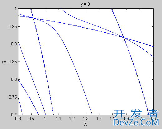
Notice that there are now additional lines in the plot that did not appear when using EZPLOT, and these lines are very jagged. You can zoom in on the crossing at the top left and make a plot using SURF to get an idea of what's going on:

lambda = linspace(0.85,0.95,100);  %# Some new lambda values
betab = linspace(0.95,1,100);      %# Some new betab values
[L,B] = meshgrid(lambda,betab);    %# Create 2-D grids of values
y = f1(L,B);                       %# Evaluate f1 at every point in the grid
surf(L,B,y);                       %# Make a 3-D surface plot of y
axis([0.85 0.95 0.95 1 -5000 5000]);                 %# Change the axes limits
xlabel('\lambda');                                   %# Add an x label
ylabel('$\overline{\beta}$','Interpreter','latex');  %# Add a y label
zlabel('y');                                         %# Add a z label

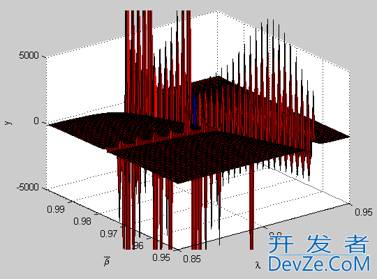
Notice that there is a lot of high-frequency periodic activity going on along those additional lines, which is why they look so jagged in the contour plot. This is also why a very general utility like EZPLOT was displaying a break in the lines there, since it really isn't designed to handle specific cases of complicated and poorly behaved functions.

EDIT: (response to comments)

These additional lines may not be true zero crossings, although it is difficult to tell from the SURF plot. There may be a discontinuity at those lines, where the function shoots off to -Inf on one side of the line and Inf on the other side of the line. When rendering the surface or computing the contour, these points on either side of the line may be mistakenly connected, giving the false appearance of a zero crossing along the line.

If you want to find a zero crossing given a value of lambda, you can try using the function FZERO along with an anonymous function to turn your function of two variables f1 into a function of one variable fcn:

lambda_zero = 1.5;             %# The value of lambda at the zero crossing
fcn = @(x) f1(lambda_zero,x);  %# A function of one variable (lambda is fixed)
betab_zero = fzero(fcn,0.94);  %# Find the value of betab at the zero crossing,
                               %#   using 0.94 as an initial guess